3D Point Clouds for Objects Using TangoCamera
In order to test pose and other algorithms for Computer Vision, having reasonably accurate 3D locations for points in 3D space is often a requirement. 3D models obtained using Structure-from-Motion provides one solution, but its often enough to have a single point cloud for an object. The procedure below describes how to obtain such a point cloud for some given object using a Tango equipped device with TangoCamera which should often be sufficent for tests where a 360 degree view of the object is not required.
-
Take a photo with TangoCamera with point clouds enabled in the settings (the default is enabled) of the object to be modelled. It is easiest if the item is isolated against a wall or if a large room is available then with nothing behind the object. It can also make it easier if some measureable frame of reference is placed in the scene, for example a ruler. In the example below two A4 pages are placed in front of the object (the width of an A4 page being 210mm).

-
Copy the 3 files created by TangoCamera from the DCIM/TangoCamera directory into a local directory using adb, Android Studio Device Explorer or via a USB mount. For the purposes of this example it is assumed the files are copied into a sub-directory called data, for example:
adb pull /sdcard/DCIM/TangoCamera
mv TangoCamera data
Also copy the python scripts from the Analysis directory into the current directory.
-
To view stats involving the point cloud use ply-analysis.py:
-h, --help           show this help message and exit
-s, --stats          Print stats
-d, --distributions  Show probability distributions for x, y and z.
--Jxy                Show joint probability distribution for x and y.
--Jxz                Show joint probability distribution for x and z.
--Jyz                Show joint probability distribution for y and z.
-b, --box            Show boxplot.
Note: requires python packages numpy, pandas, matplotlib, seaborn and plyfile. eg python ply-analysis.py data/20171122163055.165-94478.413933571.ply -s -d -b
                  x             y             z
count  25038.000000  25038.000000  25038.000000
mean      -0.005537     -0.051417      0.442446
std        0.156137      0.095564      0.096354
min       -0.277612     -0.220043      0.092123
25%       -0.133545     -0.135179      0.435486
50%       -0.017069     -0.061922      0.492052
75%        0.124652      0.052491      0.497753
max        0.289132      0.089715      0.503673
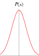
- From the distributions we can infer the most likely point ranges and use
ply-filter.py to create a modified point cloud. In this case we will filter
Z between 0.40 and 0.485 (-Z 0.40 –ze 0.485) and Y less than 0.050101
(-y 0.050101) (note the point cloud coordinate system is defined as
“+Z points in the direction of the camera’s optical axis, perpendicular to the plane of the camera.
+X points toward the user’s right, and +Y points toward the bottom of the screen. The origin is the focal center
of the depth camera.”, ie similar to OpenCV. Point cloud coordinates are in metres).
the command line for this is:
python3 ply-filter.py -i -Z 0.40 --ze 0.485 -y 0.050101 data/20171122163055.165-94478.413933571.ply -o test.ply - Finally the filtered result can be checked by projecting the 3D points onto the image
using project.py (requires numpy-quaternion and
python-opencv):
 Note the code for project.py is still experimental and a bit of a mess. In particular the projections
Y translation is off. Subtracting the translation between the color camera and the IMU
(see “Coordinate frames for component alignment”)
seems to solve it, but its only tested on a Zenfone. Regardless, the identified points should be usable where 3D
odel points are required, eg for testing PnP style pose algorithms. The command line used for the image above was:
Note the code for project.py is still experimental and a bit of a mess. In particular the projections
Y translation is off. Subtracting the translation between the color camera and the IMU
(see “Coordinate frames for component alignment”)
seems to solve it, but its only tested on a Zenfone. Regardless, the identified points should be usable where 3D
odel points are required, eg for testing PnP style pose algorithms. The command line used for the image above was:
python project.py -c y data/20171122163055.165-94478.413933571.jpg data/20171122163055.165-94478.413933571.yaml test.plyFor algorithms which have issues with co-planar points, it might be a good idea to use Z color coding, rather than the Y color coding illustrated above, to help select non co-planar points, ie change -c y to -c z in the above command line.
- The ply-display.py script can be used to view the point cloud in 3D:
python ply-display.py test.ply